Linear Equations and Matrices

• linear functions
• linear equations
• solving linear equations

Linear functions

function f maps n-vectors into m-vectors is linear if it satisfies:

• scaling: for any n-vector x, any scalar α, f(αx) = αf(x)
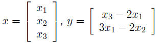
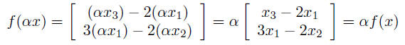
• superposition: for any n-vectors u and v, f(u + v) = f(u) + f(v)

example: f(x) = y, where

let’s check scaling property:

Matrix multiplication and linear functions

general example: f(x) = Ax, where A is m × n matrix

• scaling: f(αx) = A(αx) = αAx = αf(x)
• superposition: f(u + v) = A(u + v) = Au + Av = f(u) + f(v)

so, matrix multiplication is a linear function

converse: every linear function y = f(x), with y an m-vector and x and
n-vector, can be expressed as y = Ax for some m × n matrix A

you can get the coefficients of A from

Composition of linear functions

suppose

• m-vector y is a linear function of n-vector x, i.e., y = Ax where A is
m × n
• p-vector z is a linear function of y, i.e., z = By where B is p × m.

then z is a linear function of x, and z = By = (BA)x

so matrix multiplication corresponds to composition of linear functions,
i.e., linear functions of linear functions of some variables

Linear equations

an equation in the variables x₁, . . . , x_n is called linear if each side consists
of a sum of multiples of x_i, and a constant, e.g.,

is a linear equation in x₁, x₂, x₃

any set of m linear equations in the variables x₁, . . . , x_n can be
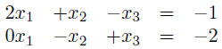
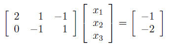
represented by the compact matrix equation

Ax = b,

where A is an m × n matrix and b is an m-vector

Example

two equations in three variables x₁, x₂, x₃:

step 1: rewrite equations with variables on the lefthand side, lined up in
columns, and constants on the righthand side:

(each row is one equation)

step 2: rewrite equations as a single matrix equation:

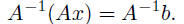
• ith row of A gives the coefficients of the ith equation
• jth column of A gives the coefficients of x_j in the equations
• ith entry of b gives the constant in the ith equation

Solving linear equations

suppose we have n linear equations in n variables x₁, . . . , x_n

let’s write it in compact matrix form as Ax = b, where A is an n × n
matrix, and b is an n-vector

suppose A is invertible, i.e., its inverse A⁻¹ exists

multiply both sides of Ax = b on the left by A⁻¹:

lefthand side simplifies to A⁻¹Ax = Ix = x, so we’ve solved the linear
equations: x = A⁻¹b

so multiplication by matrix inverse solves a set of linear equations
some comments:

• x = A⁻¹b makes solving set of 100 linear equations in 100 variables
look simple, but the notation is hiding alot of work!

• fortunately, it’s very easy (and fast) for a computer to compute
x = A⁻¹b (even when x has dimension 100, or much higher)

many scientific, engineering, and statistics application programs

• from user input, set up a set of linear equations Ax = b
• solve the equations
• report the results in a nice way to the user

when A isn’t invertible, i.e., inverse doesn’t exist,

• one or more of the equations is redundant
(i.e., can be obtained from the others)
• the equations are inconsistent or contradictory

(these facts are studied in linear algebra)

in practice: A isn’t invertible means you’ve set up the wrong equations, or
don’t have enough of them

Solving linear equations in practice

to solve Ax = b (i.e., compute x = A⁻¹b) by computer, we don’t compute
A⁻¹, then multiply it by b (but that would work!)

practical methods compute x = A⁻¹b directly, via specialized methods
(studied in numerical linear algebra)

standard methods, that work for any (invertible) A, require about n³
multiplies & adds to compute x = A⁻¹b

but modern computers are very fast, so solving say a set of 500 equations
in 500 variables takes only a few seconds, even on a small computer

. . . which is simply amazing

Solving equations with sparse matrices

in many applications A has many, or almost all, of its entries equal to zero,
in which case it is called sparse

this means each equation involves only some (often just a few) of the
variables

sparse linear equations can be solved by computer very efficiently, using
sparse matrix techniques (studied in numerical lineae algebra)

it’s not uncommon to solve for hundreds of thousands of variables, with
hundreds of thousands of (sparse) equations, even on a small computer

. . . which is truly amazing

(and the basis for many engineering and scientific programs, like simulators
and computer-aided design tools)