

Graphing and Writing Linear Functions SOLVING EQUATIONS INVOLVING RATIONAL EXPONENTS Linear Equations and Graphing Systems of Linear Equations Solving Polynomial Equations Matrix Equations and Solving Systems of Linear Equations Introduction Part II and Solving Equations Linear Algebra Graphing Linear Inequalities Using Augmented Matrices to Solve Systems of Linear Equations Solving Linear Inequalities Solution of the Equations Linear Equations Annotated Bibliography of Linear Algebra Books Write Linear Equations in Standard Form Graphing Linear Inequalities Introduction to Linear Algebra for Engineers Solving Quadratic Equations THE HISTORY OF SOLVING QUADRATIC EQUATIONS Systems of Linear Equations Review for First Order Differential Equations Systems of Nonlinear Equations & their solutions LINEAR LEAST SQUARES FIT MAPPING METHOD FOR INFORMATION RETRIEVAL FROM NATURAL LANGUAGE TEXTS Quadratic Equations Syllabus for Differential Equations and Linear Alg Linear Equations and Matrices Solving Linear Equations Slope-intercept form of the equation Linear Equations DETAILED SOLUTIONS AND CONCEPTS QUADRATIC EQUATIONS Linear Equation Problems Systems of Differential Equations Linear Algebra Syllabus Quadratic Equations and Problem Solving LinearEquations The Slope-Intercept Form of the Equation Final Exam for Matrices and Linear Equations Linear Equations |
Introduction Part II and Solving Equations1 Numerical Solution to Quadratic EquationsRecall from last lecture that we wanted to find a numerical solution to a quadratic equation like
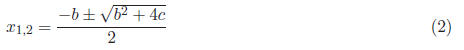
One obvious attempt at a solution would use the familiar quadratic formula:
But, while it is trivial for a computer to perform additions, subtractions,
multiplications, and 2 Finding Square Roots and Solving Quadratic Equations2.1 Finding Square Roots As we discussed last time, there is a simple scheme for approximating square
roots to any given
using an iterative method that allows us to control the precision of the
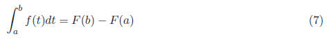
solution. The idea is that
An interesting property of this algorithm is that the precision of the output
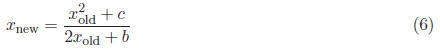
(xnew) doubles the 2.2 Solving Quadratic Equations Now that we have a scheme for solving a restricted kind of quadratic
equation, can we use the
We simply need to add another term to the denominator of the formula:
We can use this new formula iteratively to arrive at numerical solutions of
the quadratic equation So, it should now be clear that algorithms that are good for finding
numerical solutions are 3 Calculating Definite IntegralsAnother good example of the difference between numerical computation and
analytic solutions is
Figure 1: The Definite Integral of f(t) over [a, b] What is the best way to calculate the definite integral? Our experience in
math classes suggests
But this brings up two important questions: 2. How difficult is it to evaluate the anti-derivative function at a and b? The answer to question 1 may seem simple - we all learned to calculate
anti-derivatives in
So is there a method for calculating the definite integral that uses only
information we already
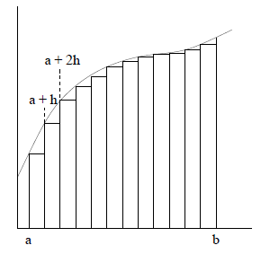
Figure 2: Approximating the Definite Integral Using Subintervals We have reduced the problem to estimating the definite integral over smaller
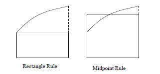
subintervals. Here Rectangle Rule
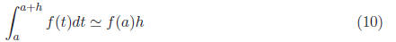
In the rectangle rule, we calculate the area of the rectangle with width h
and height determined Midpoint Rule
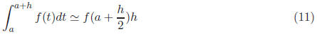
In the midpoint rule, we calculate the area of the rectangle with width h and
height determined
Figure 3: The Rectangle and Midpoint Rules These two methods are depicted in Figure 3. Using these methods, we can
calculate the definite 3.1 Evaluating Numeric Algorithms In general, we evaluate numeric algorithms using 3 major criteria: Cost - The amount of time (usually calculated as the number of operations)
the computation will Speed - How quickly the algorithm approaches our desired precision. If we
define the error as the Robustness - How the correctness of the algorithm is affected by different
types of functions and different 3.2 Evaluation of Algorithms for Definite Integrals Applying these criteria to the midpoint and rectangle rules: Cost Each algorithm performs a single function evaluation to estimate
the definite integral over a Speed Clearly as the size of each subinterval h gets smaller, the
error gets smaller as well. Is there Rectangle Rule -For the rectangle rule, the error approaches 0 in direct
proportion to the Midpoint Rule -For the midpoint rule, the error approaches 0 in
proportion to the rate at Robustness It turns out that for functions that are reasonably
well-behaved, these methods are Through this evaluation, we have shown that, in general, the midpoint rule is
a far better choice 4 Loss of SignificanceOne final way that numerical computation is different than the way you have
done mathematics to π = 3.1415926535 If we subtract π from b, we will get the answer 0.0000000036, which has only
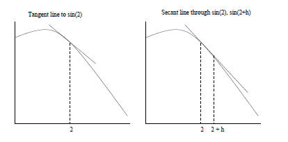
two significant Example 4.1 (Calculating Derivatives). Given the function f(t) = sin t, what is f′(2)? We all know from calculus that the derivative of sin t is cos t, so one could
calculate cos(2) in Instead, recall that the value of the derivative of a function f at a fixed
point t0 is the slope
Just as with the definite integral, we could approximate the derivative at t0
by performing Preventing loss of significance in our calculations will be an important part of this course.
Figure 4: Tangent and Secant Lines on f(t) = sin t 5 Solving EquationsNow that we have some idea of what algorithms for computation are, we will
discuss algorithms
Figure 5: Graphical Solution for x^3 = sin x Consider the following equation, with solution depicted in Figure 5.
There is no analytic solution to this equation. Instead, we will present an
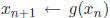
iterative method for 5.1 Iterative Method As in our solution to finding square roots, we would like to find a function
g, such that if we input Clearly, one property of g is that g(r) = r, where r is the real solution to
Equation 13. A |


 f(t)dt
is the area under the
f(t)dt
is the area under the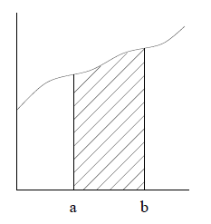

 we can calculate
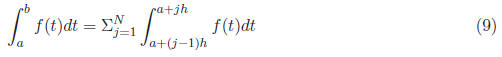
 for some fixed constant
 .
For example, halving the size of h will halve the amount of error.
.
For example, halving the size of h will halve the amount of error. for some fixed constant
 .
For example, halving the size of h will divide the error by 4.
.
For example, halving the size of h will divide the error by 4.

 with
with
 such that


