

Graphing and Writing Linear Functions SOLVING EQUATIONS INVOLVING RATIONAL EXPONENTS Linear Equations and Graphing Systems of Linear Equations Solving Polynomial Equations Matrix Equations and Solving Systems of Linear Equations Introduction Part II and Solving Equations Linear Algebra Graphing Linear Inequalities Using Augmented Matrices to Solve Systems of Linear Equations Solving Linear Inequalities Solution of the Equations Linear Equations Annotated Bibliography of Linear Algebra Books Write Linear Equations in Standard Form Graphing Linear Inequalities Introduction to Linear Algebra for Engineers Solving Quadratic Equations THE HISTORY OF SOLVING QUADRATIC EQUATIONS Systems of Linear Equations Review for First Order Differential Equations Systems of Nonlinear Equations & their solutions LINEAR LEAST SQUARES FIT MAPPING METHOD FOR INFORMATION RETRIEVAL FROM NATURAL LANGUAGE TEXTS Quadratic Equations Syllabus for Differential Equations and Linear Alg Linear Equations and Matrices Solving Linear Equations Slope-intercept form of the equation Linear Equations DETAILED SOLUTIONS AND CONCEPTS QUADRATIC EQUATIONS Linear Equation Problems Systems of Differential Equations Linear Algebra Syllabus Quadratic Equations and Problem Solving LinearEquations The Slope-Intercept Form of the Equation Final Exam for Matrices and Linear Equations Linear Equations |
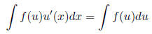
Review for First Order Differential Equations1 Integration techniques1.1 Integration by substitution
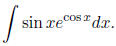
Example:
Example:
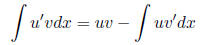
1.2 Integration by parts
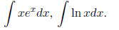
Example:
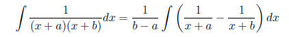
1.3 Integration by partial fractions
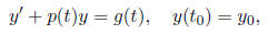
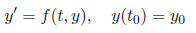
2 Existence and uniqueness2.1 Linear Equations For initial value problem
if •the coefficients p(t) and g(t) are both continuous on (a,b), and then the initial value problem has a unique solution on the entire (a, b). (Theorem 2.1) The general procedure to find such an interval (a, b) for the existence of a
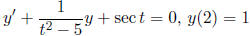
unique solution Example: For initial value problem
2.2 Nonlinear equations For initial value problem
if •f(t, y) and fy(t, y) are both continuous on the open rectangle R
defined by a < t < b •(t0, y0) is in R, then there is an open t-interval (c, d), contained in (a, b) and containing t0
(i.e., a ≤ c < Note that: 1. Theorem 2.2 doesn’t give the exact numbers for (c, d), 2.
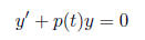
Theorem 2.2 3 First order linear differential equations3.1 Homogeneous equations
General solution is
where c is a constant and
3.2 Nonhomogeneous equations
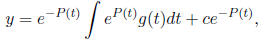
General solution is
where the first term is a particular solution to the nonhomogeneous equation,
and the You should know how to use integrating factor μ(t) = eP(t) to turn the left hand
side Example: Solve
4 First order nonlinear differential equationsIn this course we only need to know how to solve the separable equations
Example: Solve
Example: Solve
5 Applications5.1 Mixing problems
Generally, the outflow is well mixed:
5.2 Radioactive decay
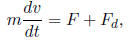
5.3 1D motion with drag force
where F is the driving force such as gravity, Fd is the drag force. 1. Drag force proportional to velocity: Fd = -kv. 5.4 1D motion with distance as the independent variable In 1D motion, if x(t) is a monotonic function (one-to-one), then velocity can
be expressed
This transformation from v(t) to v(x) is especially useful when the forcing
term is x dependent. 6 Euler’s MethodIn real applications, most equations we have to solve don’t have analytical
solutions. In
we use the following recursive procedure
Here h is the step size and
|

 1,Find
the largest
1,Find
the largest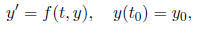
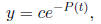
 is the antiderivative of p(t).
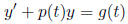


 , where V is the volume of the container.
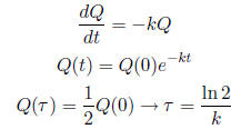
 if
if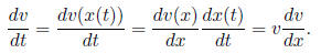

 Please note that the sequence (y1, y2, … ) is only