
Graphing and Writing Linear Functions SOLVING EQUATIONS INVOLVING RATIONAL EXPONENTS Linear Equations and Graphing Systems of Linear Equations Solving Polynomial Equations Matrix Equations and Solving Systems of Linear Equations Introduction Part II and Solving Equations Linear Algebra Graphing Linear Inequalities Using Augmented Matrices to Solve Systems of Linear Equations Solving Linear Inequalities Solution of the Equations Linear Equations Annotated Bibliography of Linear Algebra Books Write Linear Equations in Standard Form Graphing Linear Inequalities Introduction to Linear Algebra for Engineers Solving Quadratic Equations THE HISTORY OF SOLVING QUADRATIC EQUATIONS Systems of Linear Equations Review for First Order Differential Equations Systems of Nonlinear Equations & their solutions LINEAR LEAST SQUARES FIT MAPPING METHOD FOR INFORMATION RETRIEVAL FROM NATURAL LANGUAGE TEXTS Quadratic Equations Syllabus for Differential Equations and Linear Alg Linear Equations and Matrices Solving Linear Equations Slope-intercept form of the equation Linear Equations DETAILED SOLUTIONS AND CONCEPTS QUADRATIC EQUATIONS Linear Equation Problems Systems of Differential Equations Linear Algebra Syllabus Quadratic Equations and Problem Solving LinearEquations The Slope-Intercept Form of the Equation Final Exam for Matrices and Linear Equations Linear Equations |
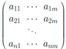
Systems of Differential Equations1 Matrices and Systems of Linear EquationsAn n × m matrix is an array A = (aij) of the form
where each aij is a real or complex number.
is called the j−th column of A and the 1×m matrix
is called the i − th row of A.
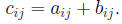
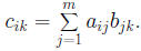
We can multiply an n × m matrix A = (aij) by an
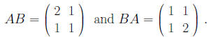
Thus the element cik is the dot product of the ith row (A + B) + C = A + (B + C), (AB)C = A(BC). Multiplication of n×n matrices is not always commutative.
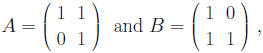
then,
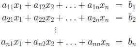
We will write vectors x = (x1, . . . , xn) in Rn both as Since our interest here is in treating systems of differential
as a single vector equation where A in the n × n matrix (aij), x is an unknown AI = IA = A. An n × n matrix A is invertible if there is another The matrix B is unique and called the inverse of A.
with the
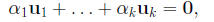
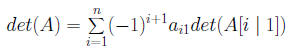
Ax = b Fact. The following conditions are equivalent for an 1. the rows of A form a linearly independent set of vectors We define the number det(A) inductively by
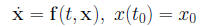
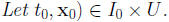
where A[i | 1] is the (n−1)×(n−1) matrix obtained 2 Systems of Differential EquationsLet U be an open subset of Rn, I be an open interval in
is called a first order ordinary differential equation in
where t0 ∈I and x0 ∈U.
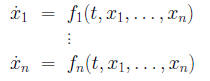
for t ∈J. x(t, c) (3) where c is an n−dimensional constant vector in Rn If we write out the D.E. (1) in coordinates, we get a
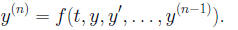
Fact: The n−th order scalar D.E. is equivalent to a Consider
Letting
If we have a solution y(t) to (5), and set x1 = y(t), x2(t) = The following existence and uniqueness theorem is proved Theorem (Existence-Uniqueness Theorem for
If the right side of the system f (t, x) does not depend
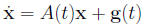
where f is a C1 function defined in an open subset U 2.1 Linear Systems of Differential Equations: General The system
in which A(t) is a continuous n × n matrix valued As in the case of scalar equations, one gets the general
Then, one finds a particular solution xp(t) to (8) and
Accordingly, we will examine ways of doing both tasks. Let yi(t) be a collection of Rn−valued functions for
for all t, we have that
A necessary and sufficient condition for the matrix If y1(t), . . . , yn(t) are n solutions to (9), and
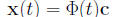
is called the Wronskian of the collection {y1(t), . . . , yn(t)} The general solution to (9) has the form
where
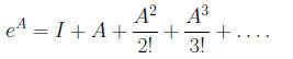
Thus, we have to find fundamental matrices and particular To close this section, we observe an analogy between
and the scalar equation x' = ax.
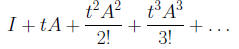
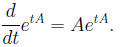
It can be shown that the matrix series on the right In particular, for a real number t, the matrix function
term by term satisfies
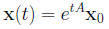
It follows that, for each vector x0, the vector function
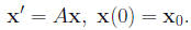
is the unique solution to the IVP
Hence, the matrix etA is a fundamental matrix for the
This observation is useful in certain circumstances,
|


 constants (scalars) we must have

 containing t0 such
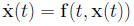
 we get
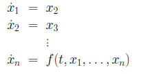
 Then, there is a unique solution
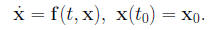


 are k scalars
 of linearly independent solutions

 is a differentiable matrix valued funtion and its